Aspen Gulley

---

In this project, I will present the fundamental principles of structural equation modeling while showcasing multiple examples along the way. I will outline the five steps involved in SEM and explain the importance parsimony. I will then provide some examples of implementing SEM in R. These examples will demonstrate how to specify, fit, and inspect the models. I will also review how to compare models using ANOVA and provide guidance on model modification. Lastly, I will demonstrate how to implement a latent growth model.

Structural equation modeling is a statistical method used to test the relationships between observed and unobserved variables (Civelek, 2017, p. 6).

This is an example of a structural equation model.

In this model the observed variables, also known as manifest variables, are represented by the rectangles. These observed variables map to an unobserved variable, otherwise known as a latent construct.

The latent constructs of motivation, stress, and positivity, all of which cannot be observed directly, were measured on a 5-point Likert Scale by 3 survey statements.

The latent construct language was measured by the scores on 5 tests, including grammar, vocabulary, comprehension, situational writing task fulfillment and situational writing language.

The question being explored is: How do the three constructs of motivation, stress, and positivity affect the construct of language ability?

Now that I have introduced SEM, I want to explore why it is interesting.

SEM is interesting because it provides a framework for analyzing complex relationships between variables in a model. What is particularly interesting about SEM is that it can be used to study the relationships of unobservable constructs. Additionally, it can measure both the direct and indirect effects between variables. A direct effect refers to how one variable directly influences another, while an indirect effect refers to the effects that one variable can have on another while being mediated by other variables in the model.

Another characteristic that makes SEM interesting is that it can be applied to a wide variety of domains where the relationship between variables are of interest. For example, SEM is useful in the medical and behavioral sciences where latent constructs such as health-related quality of life, treatment adherence, health-risk behavior, personality traits, self-efficacy, attitudes, well-being etc. can be studied. It is also beneficial in economics where it can be used to measure constructs such as consumer behavior and financial risk. SEM is also commonly used in ecology where it can be used to explore biodiversity, habitat quality, nutrient cycling, ecological resilience, etc. SEM is used in education to model the relationships between academic interventions and outcomes, among other things. Other fields where SEM is often utilized include sociology, marketing, political science, and social work.

SEM can accommodate multiple data types, which makes it flexible, and it allows researchers to evaluate how hypothetical models fit the data. This process can lead to model refinement and validation, as well as the generation of new hypothesis.

Another characteristic that makes SEM interesting is that it can be used for both longitudinal analysis and latent growth modeling. Longitudinal studies can model behavior changes over time. This can be helpful in psychology when researchers are interested in behavioral developmental trajectories. Latent growth models can be used to research growth trajectories over time. For example, the latent variable of academic performance could be studied over the course of various semesters using the manifest variable of GPA.

To summarize, SEM is a flexible framework for examining hypothesized causal relationships between variables by estimating the extent that one variable influence another while controlling for other variables in the model.

It is important to note that, generally, SEM does not test causal relationships directly, instead, it provides evidence supporting the hypothesis of causality.

For causation to be determined several conditions are required.

“There must be an empirical association between the variables — they are significantly correlated. A common cause of the variables has to be ruled out, and the two variables have a theoretical connection. Also, one variable precedes the other, and if the preceding variable changes, the outcome variable also changes (and not vice versa). These requirements are unlikely to be satisfied; thus, causation cannot be definitively demonstrated.” (Beran & Violato, 2010, p. 8).

SEMS contains both endogenous and exogenous variables. In this example the language latent variable is endogenous and the three exogenous variables are motivation, stress, and positivity.

Endogenous variables are “dependent variables explained by other variables” (Civelek, 2017, p.18). In this example, language is being explained by motivation, stress, and positivity.

Exogenous variables are “independent” and “not explained by other variables” (Civelek, 2017, p.18).

Notice in this model that the exogenous variables are related by double headed arrows. These double headed arrows represent covariance between the exogenous variables. This covariation occurs due to factors external to the model. For example, motivation might be influenced by the educational system, social environment, incentives, etc. Stress might be influenced by external factors such as the home environment, socioeconomic status, or other life events. Positivity could be influenced by culture, personal well-being, environmental factors, such as what media someone is exposed to, etc.

The endogenous variable language is influenced by motivation, stress, and positivity, and these relationships are represented by the single arrow head pointing from each of those variables to language. This single head arrow represents regression paths.

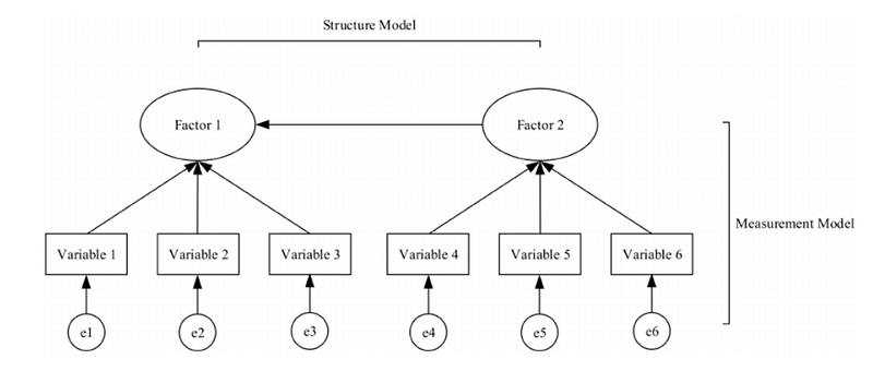
In this simple example, notice that Factor 2 is exogenous, and Factor 1 is endogenous. There is a regression path from Factor 2 to Factor 1. The rectangle variables represent the manifest variables, which are observed, and could be questions on a research survey, for example. The error circles contributing to the manifest variables represent measurement error or unobserved variability, which accounts for the portion of the observed variable that is not explained by the latent variable.

Also notice that the model has two parts, the structural model and the measurement model.

The structural model accounts for the hypothesized causal relationships between the latent variables, while the measurement model accounts for how well the latent constructs are measured by the manifest variables. The manifest variables should be reliable and valid measurements of the latent variable.

Factor loadings are used to represent the correlation between the manifest variable and the latent variable. For example, a factor loading of 0.7 would imply that 49% (0.7²) of the manifest variable’s variance is accounted for by the latent variable.

The basic mathematical goal behind SEM is to use regression to estimate a set of equations that describe the relationships between variables. Essentially, we want to know how the changes in one variable are associated with the changes in another variable. These changes are represented as path coefficients which indicate the strength and direction of the relationships.

The SEM equation can be written in matrix notation: Y = B * X + E. In this equation Y is a vector of observed variables. X is a vector of latent variables. B is a matrix of regression coefficients that describe the relationship among the variables. E is a vector of error terms that represent the unexplained variance in Y. The parameters of B and X are what SEM is trying to estimate, typically through maximum likelihood estimation.

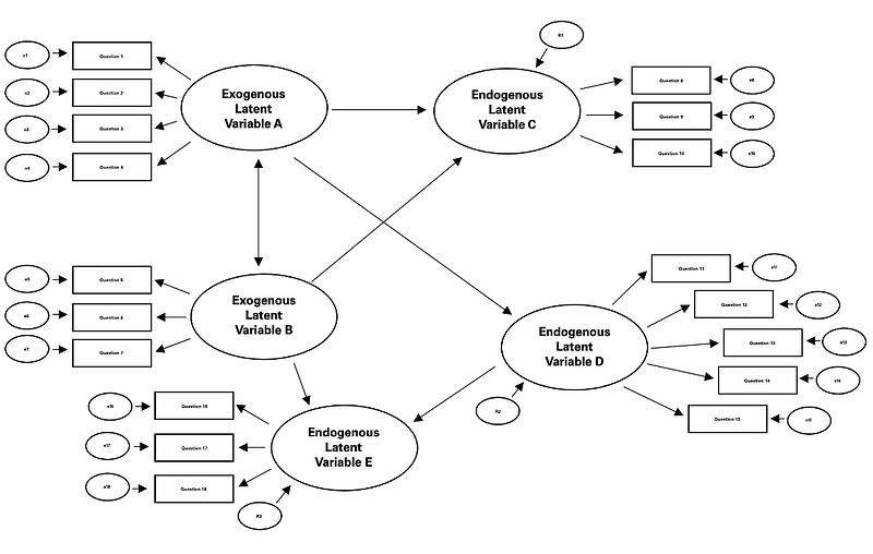
This SEM demonstrates an example of the mathematics. In this example the components of the SEM are clearly labeled. The oval latent variables are measured by the rectangle manifest variables. Measurement error of the observed variables is accounted for, as well as the residual error of the latent variables. This represents the unexplained variability in the endogenous latent variable that is not accounted for by the model. The double arrow represents covariance between the exogenous variables while the single headed arrow represents the regression path from the exogenous variable to the endogenous variable.

The regression equations for the SEM are demonstrated.

In the first equation for the variable C, 𝛽₁ and 𝛽₂ represent the path coefficients. These indicate the strength and direction of the relationship between variables C and A, as well as C and B. Res₁ represents the residual error that accounts for the unexplained variability in C that is not captured by variables A and B.

Equations for endogenous variables D and E are similarly self-explanatory.

Q1 represents the relationship between the observed variable Question 1 and the latent exogenous variable A. Lambda is the factor loading (or path coefficient) between the latent variable A and the manifest variable Question 1. It indicates the strength and direction of that relationship. As previously mentioned, the factor loading accounts for how much of the manifest variable’s variance is accounted for by the latent variable. 𝐴 in the equation represents the latent exogenous construct that is inferred from the manifest variables. 𝑒₁ is the error term which represents the unexplained variability, or measurement error, in Question 1. In summary, the manifest variable Question 1 is influenced by the exogenous latent variable A through the factor loading Lambda 1, while measurement error is also being accounted for.

The equation examples for the manifest variables similarly self-explanatory.

Here is an applied example of the SEM regression equations. In this example Health Promoting Leadership is an exogenous variable, while Resources, Stress, and Burnout are endogenous.

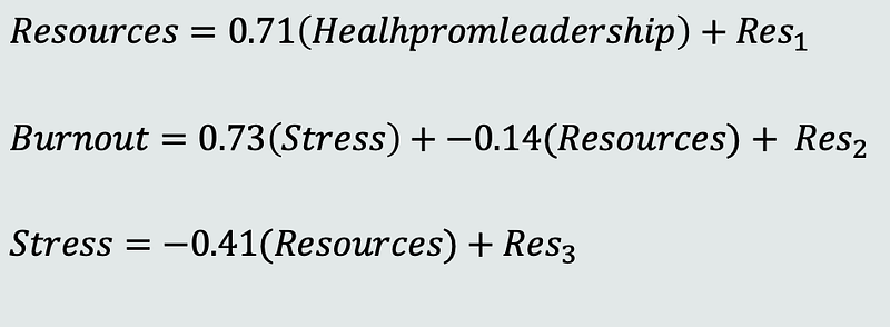
In the first equation the relationship between Resources and Health Promoting Leadership is represented. The path coefficient 0.71 represents the factor loading, and it indicates a positive relationship. Residual 1 represents the unexplained variability.

In the second equation the relationship between Burnout and two latent variables, Stress and Resources, is represented. The path coefficient 0.73 represents the factor loading between Stress and Burnout, while the path coefficient -0.14 represents the factor loading between Resources and Burnout. A positive relationship between Stress and Burnout is indicated, while a negative relationship is indicated between Resources and Burnout. Residual 2 accounts for the unexplained variability.

In the third equation the relationship between Stress and Resources is represented. The path coefficient -0.41 represents the factor loading and indicates a negative relationship. Residual 3 accounts for the unexplained variability.

There are several different types of structural equation models. They differ in the relationships they examine and their purpose.

Path analysis is a type of regression “whereby the equations representing the effect of one or more variables on others can be solved to estimate their relationships” (Beran & Violato, 2010, p. 2). Path analysis can account for multiple predictor variables, and it examines the strength of relationships between variables and their direct and indirect effects on an outcome variable.

Confirmatory factor analysis is used to test the validity of a predetermined hypothesized model, usually based on theory and prior research. It explores the degree to which the manifest variables are related to their latent construct. If confirmatory factor analysis provides evidence that the model is valid, researchers can then hypothesize the relationships between the latent variables in the SEM.

The graphic shows this process. The only relationships modeled in confirmatory factor analysis are between the manifest and latent variables. After the conversion, the SEM displays the additional relationships between the latent variables.

Structural regression models combine confirmatory factor analysis and multiple regression. Confirmatory factor analysis is used to validate the hypothesized model and then multiple regression is used to estimate the direct effects of latent variables on the outcome. According to Civelek 2017 One benefit of structural regression models are that they allow “the inclusion of measurement errors so that more accurate results can be obtained” (Civelek, 2017, p. 6).

Latent change models are used to examine changes in latent variables over time. For example, a psychologist might use this model to study how the personality changes over time. In latent change models there are two developments, a growth process, and a measure process. The growth process represents how the latent variables changes and the measure process represents the measurements at various points in time.

SEM is a flexible methodology, and it can accommodate a variety of data types. Some of these include continuous, discrete, ordinal, categorical, and latent variables.

There are several assumptions that should be considered when performing SEM. The observed variables should have multivariate normality. This means that each variable should be normally distributed, and the joint distribution of the variables should be normal. The endogenous latent variables should also have a multivariate normal distribution. When normality assumptions are violated robust maximum likelihood estimation or weighted least squares are estimation methods that could be considered as alternative options. A linear relationship between the manifest and latent variables is assumed, as well as a linear relationship between the latent variables (Civelek, 2017). Because the linear relationship is assumed, there should not be outliers impacting the accuracy of predictions. At least three or more observed variables should measure one latent variable. There should not be relations among the independent variables. An adequate samples size is needed. Error terms should not be correlated “unless explicitly stated by the researcher in the conceptual model” according to Civelek 2017 (Civelek, 2017, p.31).

Not all of these assumptions are relevant for every structural equation model and at times some of the assumptions can be relaxed. For example, there are instances when normality assumption is violated, and the structural equation model results are still valid. In general, it is important to consider these assumptions when building structural equation models.

Two common challenges that researchers face when working with this methodology includes model misspecification and acquiring adequate sample sizes.

Misspecification occurs when the theoretical model is not a good fit for the data, or model assumptions are violated. Researchers often use model modification and comparison to address this problem.

As mentioned, SEM is commonly used in a variety of domains. Some of the domains, such as the behavioral sciences, often struggle to obtain large sample sizes. Without a large enough sample size, it can be difficult to obtain a stable estimate of a complex model. Bootstrapping and Monte Carlo methods are remedies researchers utilize to address this challenge.

There are five recommended steps to follow when building a structural equation model.

Step 1: Identify the Research Problem

The first step when building a SEM, is to identify the research problem. The research problem should be specific and well-defined.

During this step, the relationships between the variables will need to be hypothesized using theory and previous research. “These relationships may be direct or indirect whereby intervening variables may mediate the effect of one variable on another. The researcher must also determine if the relationships are unidirectional or bidirectional, by using pervious research and theoretical predictions as a guide.” (Beran & Violato, 2010, p. 2).

There are several factors to take into consideration during this step. 
 
 The problem should be grounded in a theoretical framework. The variables of interest should be clearly identified. The hypothesis and research questions should be stated. The availability of data and the practical relevance of the research should also be considered. 
 (Suhr, 2006).

Step 2: Identify the Model

A model is identified when there are enough manifest variables to measure the latent variables. This occurrence is indicated when the degrees of freedom (df) are equal to or greater than 1. The number of manifest variables represent the number of possible estimates, and the latent variables represent the number of estimates that occur. The congeneric model is a “simple heuristic yields the correct answer in the typical case” (Rigdon, 1994, p. 275). This equation and an example are represented here:

For further examples and a more in-depth exploration I recommend Edward E. Rigdon’s paper, Calculating Degrees of Freedom for a Structural Equation Model.

Step 3: Estimate the Model

Estimation can be accomplished by using statistical methods to find the values of parameters that best fit the observed data. Maximum likelihood estimation is often the default method used in SEM.

“Maximum likelihood estimation (MLE) is a technique used for estimating the parameters of a given distribution, using some observed data. For example, if a population is known to follow a normal distribution but the mean and variance are unknown, MLE can be used to estimate them using a limited sample of the population, by finding particular values of the mean and variance so that the observation is the most likely result to have occurred.” (Brilliant.org, 2023, para 1)

Step 4: Determine the Model’s Goodness of Fit

According to Preacher (2006), “Goodness of fit is the empirical correspondence between a model’s predictions and observed data. If the match between the model’s predictions and observed data is deemed adequate (by reaching or exceeding some benchmark), the model is said to show good fit, an indication that the theory represented by the model has received support” (p. 231).

Various measures are used to assess the goodness of fit of a SEM. It is recommended to consider several measures when determining the model’s goodness of fit.

The “comparative fit index is most commonly used and compares the existing model with a null model” (Beran & Violato, 2010, p. 4). A good fit is indicated by a value > 0.90. The root mean square error of approximation is another commonly used fit index. This is the square root of the mean differences between the estimate and true value (Beran & Violato, 2010, p. 4). A good fit is indicated by a value less than 0.05. The standardized root mean square residual measures the discrepancy between the model-implied covariance matrix and the observed covariance matrix. A good fit is usually indicated by a value less than 0.09. The Tucker-Lewis index measures the degree to which the proposed model fits the observed data, relative to a baseline model. A value greater than 0.90 is indicative of a good fit.

Step 5: Re-specify the Model If Necessary

SEM is often an iterative process. “To obtain improved fit results” it is recommended that “the above sequence of steps is repeated until the most succinct model is derived (i.e., principle of parsimony)” (Beran & Violato, 2010, p. 5). Look for large, standardized residuals that may indicate an inadequate fit. If this is the case, adding path links or including mediating or moderating variables are some potential recommended remedies (Beran & Violato, 2010). Once an adequate fit is found, the results should be confirmed on an alternate data sample to “strengthen confidence in the inferences” (Beran & Violato, 2010, p. 5).

The next example will demonstrate an application of the 5 step SEM process.

Dr. Alla Skomorovsky and Dr. Sonya Stevens’ 2013 paper on testing a resilience model among Canadian forces recruits showcases the application of a SEM in research. According to Skomorovsky and Stevens, “some military personnel exposed to war related stressors experience no negative health consequences” and personal characteristics might be one of the variables contributing to this resilience (p. 829). 
 
 Testing a resilience model, Skomorovsky and Stevens administered questionnaires to 200 candidates in their Basic Officer Training course. Measures on this questionnaire included coping mechanisms, neuroticism, hardiness levels, life satisfaction, and general health. They “hypothesized that neuroticism (-), military hardiness (+), problem-focused coping (+), and maladaptive emotion-focused coping (-) would jointly predict life satisfaction and general health of the CF candidates” (Skomorovsky & Stevens, 2013, p. 830).

Model 1, the full model, represented all paths between the manifest and latent variables. In this model an adequate fit was indicated with the comparative fit index at 0.91 and a root mean square error of approximation at 0.06. The paths between military hardiness and general health, problem-focused coping and life satisfaction, maladaptive emotional coping and life satisfaction, and maladaptive emotional coping and general health were not significant (Skomorovsky & Stevens, 2013). All other path loadings and factor correlations were significant.

Model 2 only retained the significant paths from Model 1. “All path loadings and factor correlations were significant (Skomorovsky & Stevens, 2013, p. 834). In this model an adequate fit was indicated with the comparative fit index at 0.912 and a root mean square error of approximation at 0.059.

“In Model 3, maladaptive coping was deleted, and only neuroticism, problem-focused coping, and military hardiness predicted life satisfaction and general health” (Skomorovsky & Stevens, 2013, p. 834). Additionally, in Model 3 the paths between military hardiness and general health, and problem-focused coping and life satisfaction were not significant (Skomorovsky & Stevens, 2013). In this model an adequate fit was indicated with the comparative fit index at 0.910 and a root mean square error of approximation at 0.063.

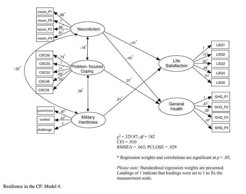
In Model 4 “maladaptive coping was deleted, and only the significant paths were retained” (Skomorovsky & Stevens, 2013, p. 834). “All path loadings and factor correlations were significant” (Skomorovsky & Stevens, 2013, p. 834). In this model an adequate fit was indicated with the comparative fit index at 0.910 and a root mean square error of approximation at 0.063.

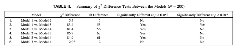
In Table I, all of the models have similar fit indices, and it is not clear if one model is a better fit than all others (Skomorovsky & Stevens, 2013).

Skomorovsky & Stevens (2013) performed chi-square difference tests to “confirm that neither model was a significantly better fit” (p. 834). The model results showed that the “maladaptive coping variable was irrelevant”, and at the 0.01 significance level the only significant difference found was between the Models 1 and 3. With the irrelevance of maladaptive coping and no significant difference between Models 3 and 4, Model 4, the most parsimonious, was retained (Skomorovsky & Stevens, 2013).

The results of this study confirmed that “neuroticism, military hardiness, and problem focused coping behaviors are important concepts that should be taken into account when explaining the variance in resilience among military personnel” (Skomorovsky & Stevens, 2013, p. 834). All of the models demonstrated that “individuals with lower neuroticism were more likely to have better resilience, when measured by life satisfaction and general health” (Skomorovsky & Stevens, 2013, p. 834). Additionally, “military hardiness was found to be an important predictor of resilience”, and those who demonstrated problem-focused coping had “better health symptoms” (Skomorovsky & Stevens, 2013, p. 834).

Skomorovsky & Stevens (2013) suggest that selecting candidates with lower neuroticism may be helpful in the “military context, because of its potentially stressful demands” (p. 835). They also recommend providing resilience training that incorporates hardiness and healthy coping mechanisms (Skomorovsky & Stevens, 2013).

Skomorovsky and Stevens (2013) demonstrate the principle of parsimony in their study by choosing the simplest model that adequately explains the data. This practice increases the likelihood that the model will generalize well to new data samples, and it decreases the risk of a Type I error (Byrne, 2016).

Skomorovsky and Stevens (2013) used hypothesis testing to compare their models. Another common approach is to examine the Akaike Information Criterion (AIC) and the Bayesian Information Criterion (BIC). These measures balance the goodness of fit and the model’s complexity. Smaller values of each indicate a better fit. It is important to note though that between the AIC and BIC, the BIC is more conservative because it imposes a larger penalty on models with increased parameters in comparison to the AIC.

With all of this in mind, and as previously stated, when evaluating and selecting a structural equation model, it is important to consider an aggregation of several measures.

Implementing Structural Equation Models in R

Before the start of any SEM project, the data needs to be prepared.

This process includes screening the data for entry errors, outliers, or missing values, and addressing each of these problems appropriately given the circumstance.

The data should meet the assumptions of normality, linearity, and homoscedasticity. The data may need to be transformed to improve distributional assumptions. The standardization or normalization of variables may also be beneficial. Potential multicollinearity should also be evaluated.

Based on the research, the specific variables appropriate for the SEM will also need to be selected and certain variables may need to be coded. For example, data from a Likert scale should be coded as ordered categorical variables.

Depending on the type of SEM, the data need may need to be organized specifically in wide or long format.

As the data is being prepared, it is also good practice to document the modifications made in preparation for the SEM.

The data used in this demonstration does not need to be prepared because it comes from the Lavaan package in the CRAN repository. These datasets include the HolzingerSwineford1939 and Demo.growth.

Starting with HolzingerSwineford1939, the data description in R says that this, “The classic Holzinger and Swineford (1939) dataset consists of mental ability test scores of seventh and eighth-grade children from two different schools (Pasteur and Grant-White).” It is a dataframe with 301 observations of 15 variables.

id: Identifier
sex: Gender
ageyr: Age, year part
agemo: Age, month part
school: School (Pasteur or Grant-White)
grade: Grade
x1: Visual Perception
x2: Cubes
x3: Lozenges
x4: Paragraph Comprehension
x5: Sentence Completion
x6: Word Meaning
x7: Speeded Addition
x8: Speeded Counting of Dots
x9: Speeded Discrimination Dtraight and Curved Capitals

Install and import the dataset into R.

#install.packages(“lavaan”)
#install.packages(“semPlot”)
library(lavaan)
library(semPlot)

The first question I am exploring is:

Does a one factor model, representing general cognitive ability, or a multiple factor model representing specific cognitive functions, fit the data better?

I am going to specify the two factor structure. The model syntax for defining a latent variable is represented with the equals and the tilde.

#Specify factor structure
model.twofactor <- ‘f1 =~ x1 + x2 + x3
f2 =~ x4 + x5 + x6′

Factor one, Visual Ability, is measured by x1: Visual Perception, x2: Cubes, and x3: Lozenges. Factor two, Textual Ability, is measured by x4: Paragraph Comprehension, x5: Sentence Completion, and x6: Word Meaning.

Next, fit the model with the confirmatory factor analysis function, and inspect the results.

#Fit model
fit.twofactor <- cfa(model.twofactor, data = HolzingerSwineford1939)

#Inspect
summary(fit.twofactor, standardize=TRUE)

By adding standardize = TRUE, the results will add standardized columns that account for differences in scale, making the output easier to interpret.

Because the results are extensive, I want to review the output before answering the question of which factor model fits the data better.

At the top of the output, the estimator is displayed. ML stands for maximum likelihood. The number or parameters being estimated is 13 and there are 301 observations in the data. The chi-square test statistic is 24.361. This is a measure of how well the model fits the data. Small chi-square values indicate a good fit. Next the degrees of freedom are presented. The nice thing about R is that is calculates the degrees of freedom for us. Because the degrees of freedom are 8, our model is identified. Remember, the degrees of freedom need to be greater than zero to be identified. The p-value is significant (less than 0.05), indicating the model fits the data well.

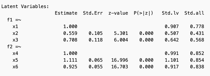
The latent variable section provides information on each latent variable and their indicator.

Looking at the standardized loadings (Std.lv) for factor one, x1: Visual Perception has a standardized loading value of 0.907. This indicates a strong positive relationship with the Visual Ability factor. This is the relationship used for reference, and so the estimate value is 1.

The positive relationship between Visual Ability and x2: Cubes is weaker than the reference, with a standardized value of 0.507.

The positive relationship between Visual Ability and x3: Lozenges is also weaker than the reference, but stronger than x2: Cubes, with a standardized value of 0.642.

The latent variable for factor 2, Textual Ability, has a strong positive relationship with x4: Paragraph Comprehension with a standardized value of 0.991. This is the reference relationship for the remaining indicators.

Textual Ability has a stronger positive relationship with x5: Sentence Completion, in comparison to x4: Paragraph Completion, as indicated by the standardized value of 1.101. Because the value is greater than one, this indicator is a stronger relationship with the factor than the reference value.

Textual Ability and x6: Word Meaning have a weaker positive relationship in comparison to both x4 and x5 with a standardized value of 0.917.

The Std.all values represent the standardized regression coefficients of the indicators on the latent variables. This represents the extent to which each indicator contributes to the latent variable, and the extent to which the indicator explains the variance of the latent variable. Higher coefficients represent stronger contributions of the indicator to the latent variable.

In this example, the standardized regression coefficient for x1: Visual Perception is 0.778, indicating that x1 contributes 77.8% to the variance of the Visual Ability factor. The standardized regression coefficient for x2: Cubes is 0.431, meaning that x2 contributes 43.1% to the variance of Visual Ability. The standardized regression coefficient value for x3: Lozenges is 0.568, indicating that x3 contributes 56.8% to the variance of Visual Ability.

For latent variable Textual Ability, the standardized regression coefficient for x4: is 0.852, indicating that x4: Paragraph Comprehension contributes 85.2% to the variance. The standardized regression coefficient x5: Sentence Completion is 0.854, meaning that x5 contributes 85.4% to the variance of Textual Ability. Lastly, the standardized regression coefficient for x6: Word Meaning is 0.838, indicating that x6 contributes 83.8% to the variance.

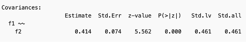
The covariance measures the relationship between the two factors by evaluating the extent to which the factors vary together. The standardized covariance estimate between the two latent factors is 0.461.

When looking at the variance results, the Std.lv values indicate the relative amount of variability in each variable. The Std.all values represent the portion of variance in each observed variable that is accounted for by the model. Higher Std.all values suggest that the model explains a larger portion of the observed variable’s variance, indicating a strong relationship between the latent variables and the observed variable.

Now that the output is understood, the question of whether a one factor model, representing general cognitive ability, or a two-factor model representing specific cognitive functions, fit the data better, can be answered.

Looking at the standardized loadings for Visual Abilities and the indicators x1-x3, (0.907, 0.507, and 0.642) it is clear there is evidence of a strong relationship between the indicators and factor one. Examining the standardized loadings for Textual Abilities and the indicators x4-x6 (0.991, 1.101, and 0.917), strong relationships between the indicators and factor two are also evident.

These results suggest that the two-factor model is appropriate. Had the loadings been small for either factor, a one factor model may have been more suitable.

I can confirm that the model fits the data well by re-running the results and adding the fit measures in the output.

#Inspect the results again, and add fit measures
summary(fit.twofactor, fit.measures=TRUE, standardize=TRUE)

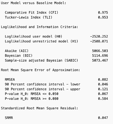
Now the results display the goodness of fit measures.

At 0.975 the comparative fit index is good because it greater than 0.90. The root mean square error of approximation is considered a good fit if the value is less than 0.05. Our value indicates a moderate fit with a value of 0.082. The standardized root mean square residual indicates a good fit at 0.047. Recall that a good fit value is less than 0.09. The Tucker-Lewis index also indicates a good fit because the value is > 0.90 at 0.953.

In combination, these results provide evidence that the two-factor model fits the data well.

I am going to run a one factor model to compare the results.

#Compare the results to a one factor model

#Specify factor structure
model.onefactor <- ‘f1 =~ x1 + x2 + x3+ x4 + x5 + x6’

#Fit model
fit.onefactor <- cfa(model.onefactor, data = HolzingerSwineford1939)

# Inspect the results
summary(fit.onefactor, fit.measures=TRUE, standardize=TRUE)

The goodness of fit measures are significantly worse.

Reviewing the standardized loadings (Std.lv), it is evident that one factor of General Cognitive Ability does not represent the relationships between latent variables and their indicators well. The measures for x2 and x3 are below 0.3, and so they are not significantly contributing to the latent variable. Moreover, the portion of explained variance in the standardized all column (Std.all) is much higher for x1-x3, compared to x4-x6.

In combination, these results support the conclusion that a two-factor model representing specific cognitive functions is more appropriate.

The next question I have is whether the factor structure remain consistent across groups.

Remember, there are two grades represented in this data, 7th and 8th, as well as two schools, Pasteur or Grant-White, and two sexes, males and females. For this example, I am going to use sex as the grouping variable. In these variables the males are represented as 1 and the females are represented as 2.

To answer this question in R, simply add group=”sex” to the confirmatory factor analysis function.

#Specify
model.groups <- ‘f1 =~ x1 + x2 + x3
f2 =~ x4 + x5 + x6′

#Fit
fit.groups <- cfa(model.groups, data=HolzingerSwineford1939, group=”sex”)

#Compare model fit indices across groups
summary(fit.groups, fit.measures=TRUE, standardize=TRUE)

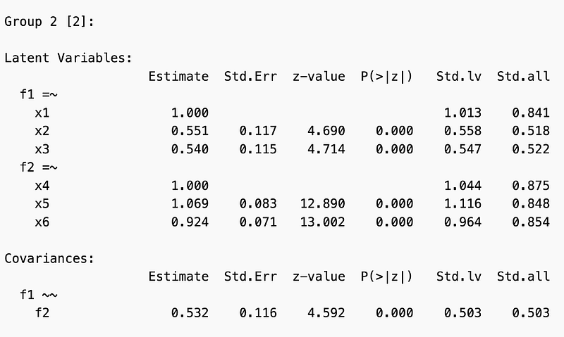
When comparing males and females, both groups have similar standardized loadings (Std.lv) on both factors. Additionally, the covariances between the factors are significant in both males and females, indicating that for both groups there is a relationship between the factors.

Despite the groups being similar, there are some differences.

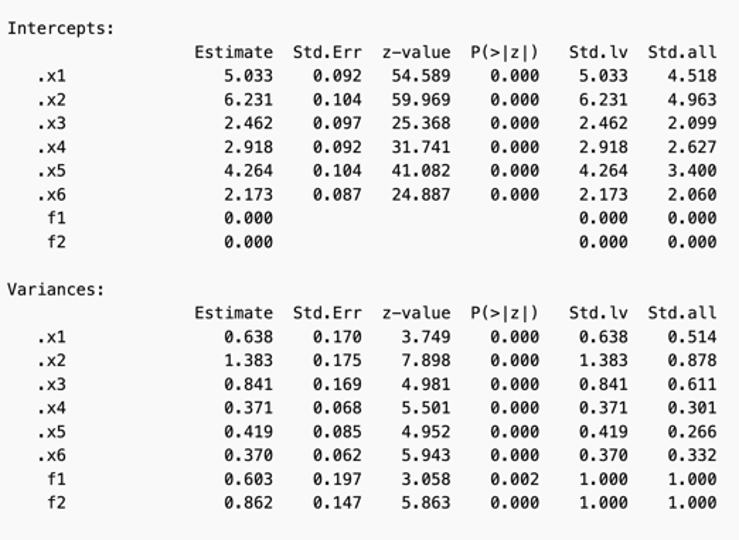
The intercepts are the average of the manifest variables when the factors are fixed at zero. When comparing the males and females, the males have higher intercepts. This indicates that the males scored higher, on average, then the females on these measures. Moreover, the variances are higher in the male group. This indicates the males had more variability in the measure responses as well.

It would be interesting to see if there are other group differences, between the schools, for example.

Can the latent factors of Visual and Textual Ability predict the observed variable grades?

I have added a regression model to the SEM. Grade represents the dependent variables and the factors represent the predictor variables.

I am using the sem() function, as opposed to cfa() because I am interested in the relationship between the latent variables and the observed variable, grade.

#Specify the model
model.predictgrades <- ‘f1 =~ x1 + x2 + x3
f2 =~ x4 + x5 + x6
grade ~ f1 + f2′

#Fit the model
fit.predictgrades <- sem(model.predictgrades, data=HolzingerSwineford1939)

#Inspect results
summary(fit.predictgrades, fit.measures=TRUE, standardize=TRUE)

Visualize the model.

quartz()
semPaths(fit.predictgrades,
what=”stand”,
fade=TRUE,
rotation=2,
style=”lisrel”,
layout=”tree2″,
curvature=3,
sizeLat=14,
sizeMan=16,
sizeMan2=5,
esize=3,
fixedStyle=5,
nCharNodes=0,
edge.color=”dodgerblue”,
edge.label.cex=1.5,
edge.label.color=”gray20″)

While both latent variables have a positive effect on the observed variable grades as indicated by the positive coefficients, only factor 1, Visual Ability, is statistically significant with a p-value less than 0.05.

With structural equation models, we can also explore questions about mediating variables. For example, is sex a mediating variable in the relationships between grades and cognitive ability?

To specify a mediating relationship between the factors and grade, the tilde is used. By specifying the direct relationship between sex and the latent factors, sex is now a mediating variable.

#Specify
model.mediating <- ‘f1 =~ x1 + x2 + x3
f2 =~ x4 + x5 + x6
grade ~ f1 + f2
f1 ~ sex
sex ~ f2′

#Fit
fit.mediating <- sem(model.mediating, data = HolzingerSwineford1939)

#Inspect
summary(fit.mediating, fit.measures=TRUE, standardize=TRUE)

#Visualize
quartz()
semPaths(fit.mediating,
what=”stand”,
fade=TRUE,
rotation=2,
style=”lisrel”,
layout=”tree2″,
curvature=3,
sizeLat=14,
sizeMan=16,
sizeMan2=5,
esize=3,
fixedStyle=5,
nCharNodes=0,
edge.color=”dodgerblue”,
edge.label.cex=1.5,
edge.label.color=”gray20″)

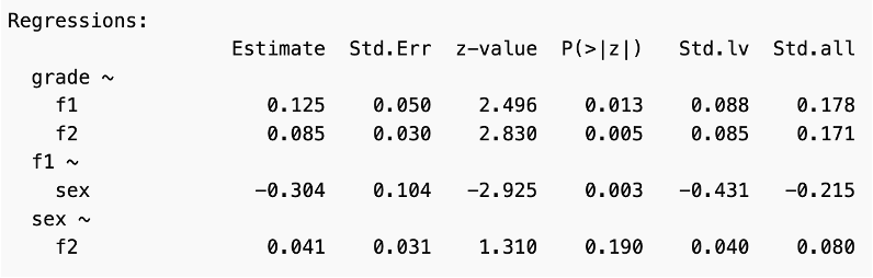
The latent factors of Visual and Textual Abilities both show a significant coefficient, and positive relationships with grade. There is a significant negative relationship between factor one, Visual Ability, and sex, indicating that it is a mediating variable. Higher values of sex, the females, are associated with lower scores on Visual Ability. Despite this, both coefficients for the factors are positive. Sex does not appear to be a significant mediating variable for Textual Ability and grade.

In the example previously reviewed of Dr. Alla Skomorovsky and Dr. Sonya Stevens’ 2013 paper on testing a resilience model among Canadian forces recruits, the 4 models had similar fit indices. I want to review how to examine whether one model is a better fit than another. To accomplish this, simply build and fit both models. Then use the ANOVA function to test the models.

#Compare models with ANOVA

model1<- ‘visual =~ x1 + x2 + x3
textual =~ x4 + x5 + x6′

fit.1 <- cfa(model1, data=HolzingerSwineford1939)

model2<- ‘visual =~ x1 + x2 + x3
textual =~ x4 + x5 + x6
x4~~x6′

fit.2 <- cfa(model2, data=HolzingerSwineford1939)

anova(fit.1, fit.2)

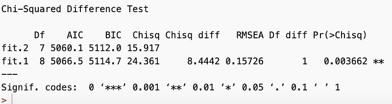
Remember, lower AIC and BIC values indicate a better fit, and fit.2 has lower values of both.

The chi-square difference between the two models is 8.4442 with a p-value is 0.003662. This indicates a statistically significant difference between the models.

When needing a roadmap to improve a models fit, the modification indices can provide some guidance. Adding sort=TRUE helps organize the modification indices from potentially most helpful to least.

modificationindices(fit.1, sort=TRUE)

The MI, modification index, column provides suggestions for model improvement. The higher the MI value, the more likely the modification is to improve the model’s fit. In this case I would add a covariance between x2: Cubes and x3: Lozenges. It is recommended to make one modification at a time and evaluate the fit measures in sequence.

Next, I want to demonstrate how to build a latent growth model.

The Demo.growth dataset in the Lavaan package is a toy dataset that can be used to illustrate a latent growth model. It is a dataframe with 400 observations and 10 variables.

t1: Measured value at time point 1

t2: Measured value at time point 2

t3: Measured value at time point 3

t4: Measured value at time point 4

x1: Predictor 1 influencing intercept and slope

x2: Predictor 2 influencing intercept and slope

c1: Time-varying covariate time point 1

c2: Time-varying covariate time point 2

c3: Time-varying covariate time point 3

c4: Time-varying covariate time point 4

# Load the Demo.growth dataset
data(Demo.growth)

#Rename variables
library(“dplyr”)

mathematical_proficiency <- Demo.growth %>% rename(“exam_1” = “t1”,
“exam_2” = “t2”,
“exam_3” = “t3”,
“exam_4” = “t4”,
“homework_completion” = “x1”,
“parental_involvement” = “x2”)

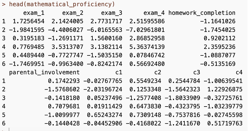
head(mathematical_proficiency)

Specify the data structure.

model.math <- ‘
intercept =~ 1*exam_1 + 1*exam_2 + 1*exam_3 + 1*exam_4
slope =~ 0*exam_1 + 1*exam_2 + 2*exam_3 + 3*exam_4
intercept ~ homework_completion
slope ~ homework_completion
intercept ~ parental_involvement
slope ~ parental_involvement’

This model explores the latent variable of mathematical proficiency. It describes how student’s exam scores change over time. The intercept represents the initial levels of exam scores. The slope represents the rate of change in exam scores over time. Each exam score is weighted differently over time, indicated by the 0, 1, 2, and 3. This shows how much each exam contributes to the growth, or change in scores. This model also includes two predictor variables, homework completion and parental involvement. The initial level of exam scores, or intercept, is impacted by the level of homework completion. The students who complete more homework are expected to have higher initial exam scores. Moreover, the slope, or rate of change in the initial exam scores, is also impacted by homework completion. The students who complete more homework are expected to have a greater increase in their exam scores over time. The same goes for parental involvement. The students who have more parental involvement are expected to have higher initial exam scores as well as a greater increase in their exam scores over time. In short, this model allows the understanding of how homework completion and parental involvement can predict the initial level and growth of the students’ exam scores.

Similar to the sem() function in previous examples, use the growth() function to fit this model.

#Fit
fit.math <- growth(model.math, data=mathematical_proficiency)

#Inspect
summary(fit.math, fit.measures=TRUE, standardized=TRUE)

The results show great goodness of fit measure with both the comparative fit index, and the Tucker-Lewis index at 0.999. The root mean square error of approximation is at 0.023 and the standardized root mean square residual is at 0.011.

In the latent variable section, the standardized factor loadings for slope grow over time. This indicates the growth component has a larger effect as time goes on. In the slope standardize all section the results also show the relationship gets stronger over time. The intercept standardized all values indicate the exam scores are significant in determining the children’s initial mathematical proficiency.

The regression results show the positive association between completing homework and higher exam scores with a standardized coefficient of 0.354. Parental involvement also indicates a positive association with exam scores, showing a standardized coefficient of 0.652.

The covariances also show a positive relationship between the intercept and slope latent variables. This shows that the students who have higher exam one scores tend to experience greater growth in their subsequent exam scores over time.

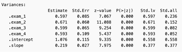
Examining the standardized all variance section, there is a decrease in variance. This suggests that there is less spread in the students’ scores as time progresses. This also suggests that at the time of exam one, there is a greater variability in the mathematical proficiency between the children compared to exam four. The intercept accounts for 0.558 of the variance in exam scores, as indicated by the standardized loadings column, while the slope accounts for 0.377 of the variance in the exam scores.

This model can be visualized as well.

quartz()
semPaths(fit.math,
what=”stand”,
fade=TRUE,
rotation=2,
style=”lisrel”,
layout=”tree”,
curvature=3,
sizeLat=8,
sizeMan=8,
sizeMan2=8,
esize=3,
fixedStyle=5,
nCharNodes=0,
edge.color=”dodgerblue”,
edge.label.cex=.5,
edge.label.color=”gray20″)

This model, measuring the latent variable of mathematical proficiency, describes how student’s exam scores change over time. The slope parameter estimates how much the latent variable changes on average for each unit of time. The slope in this model suggests that the latent variable of mathematical proficiency is exhibiting a substantial rate of change over time.

In conclusion, structural equation modeling offers a powerful toolbox for researchers. Its ability to test complex theories, analyze direct and indirect relationships between variables, and compare different models makes it a valuable tool for researchers in psychology, education, economics, public health, and many other fields. As technology continues to advance, SEM is expected to become even more crucial in analyzing complex datasets and testing hypotheses, enabling researchers to gain deeper insights into intricate variable relationships. However, it is essential to acknowledge the challenges and limitations of in SEM. These include potential model misspecification, collecting large enough sample sizes, and meeting the test assumptions. Despite these challenges, SEM provides a versatile framework for testing and refining theoretical models, guiding decision-making, and advancing research in an increasingly data-driven world.

References:

Beran, T. N., & Violato, C. (2010, October 22). Structural equation modeling in medical research: A Primer — BMC Research notes. BioMed Central. Retrieved May 5, 2023, from https://bmcresnotes.biomedcentral.com/articles/10.1186/1756-0500-3-267

Byrne, B.M. (2016). Structural Equation Modeling With AMOS: Basic Concepts, Applications, and Programming, Third Edition (3rd ed.). Routledge. https://doi.org/10.4324/9781315757421

Civelek, M. E. (2017, March 12). Essentials of structural equation modeling. digitalcommons.unl.edu. Retrieved May 3, 2023, from https://digitalcommons.unl.edu/cgi/viewcontent.cgi?httpsredir=1&article=1064&context=zeabook

Cheung, G. W. (2008). Testing Equivalence in the Structure, Means, and Variances of Higher-Order Constructs with Structural Equation Modeling. Organizational Research Methods, 11(3), 593–613. https://doi.org/10.1177/1094428106298973

Dragan, D. & Topolšek, D. (2014). Introduction to Structural Equation Modeling: Review, Methodology and Practical Applications.

Holzinger, K., and Swineford, F. (1939). A study in factor analysis: The stability of a bifactor solution. Supplementary Educational Monograph, no. 48. Chicago: University of Chicago Press.

Jiménez, P., Bregenzer, A., Kallus, K. W., Fruhwirth, B., & Wagner-Hartl, V. (2017). Enhancing Resources at the Workplace with Health-Promoting Leadership. International journal of environmental research and public health, 14(10), 1264. https://doi.org/10.3390/ijerph14101264

Joreskog, K. G. (1969). A general approach to confirmatory maximum likelihood factor analysis. Psychometrika, 34, 183–202.

Preacher, K. J. (2006). Quantifying parsimony in structural equation modeling. Multivariate Behavioral Research, 41(3), 227–259.

Maximum Likelihood Estimation (MLE). Brilliant.org. Retrieved May 17, 2023 from https://brilliant.org/wiki/maximum-likelihood-estimation-mle/)

Muthen, B. (1993). Goodness of fit with categorical and other nonormal variables. Testing Structural Equation Models. Retrieved May 5, 2023, from http://www.statmodel.com/bmuthen/articles/Article_045.pdf

Rigdon, E. (1994). Calculating degrees of freedom for a structural equation model. Structural Equation Modeling: A Multidisciplinary Journal. 1. 274–278. 10.1080/10705519409539979

Skomorovsky, A., & Stevens, S. (2013). Testing a resilience model among Canadian Forces recruits: A structural equation modeling approach. Military Psychology, 25(4), 371–382. https://doi.org/10.7205/MILMED-D-12-00389

Suhr, D. (2006). The basics of structural equation modeling. University of Northern Colorado. Retrieved May 3, 2023, from http://www.lexjansen.com/wuss/2006/tutorials/tut-suhr.pdf

Vahid Aryadoust. (2021, March 1). Statistics & Theory: Structural Equation Modeling Using AMOS [Video]. YouTube. Retrieved from https://www.youtube.com/watch?v=CxJuHqyYVGk

Ye, Jiao & Chen, Jun & Bai, Hua & Yue, Yifan. (2018). Analyzing Transfer Commuting Attitudes Using a Market Segmentation Approach. Sustainability. 10. 2194. 10.3390/su10072194.

By Aspen Gulley on June 6, 2023.